Supervised normalisation can bias microbiome analyses
Update 10/08/2023
Dr Sepich-Poore has raised some important points in an issue posted to GitHub here.
I’d like to start by thanking Dr Sepich-Poore for highlighting these issues and providing constructive feedback. I also wish to emphasize that the analysis in my blog doesn’t definitively determine the presence or absence of a cancer-specific microbial signature in the TCGA data; rather, it emphasises the importance of normalisation in microbiome studies.
The first important point raised by Dr Sepich-Poore, is that the use of Supervised Normalisation in the original TCGA paper did not include cancer type as the biological variable of interest.
Rather, sample type (Primary Tumor, Blood Derived Normal, Solid Tissue Normal etc) was used as the biological variable. The use of this variable is less likely to bias the results towards cancer type specific signatures.
However, although there are fewer variables in the sample type category, it still correlates strongly with a number of the unwanted variables. We can get a rough idea of this correlation using logistic regression.
library(tidyverse)

meta_data <- readr::read_csv("./data/tcga_metadata_poore_et_al_2020_1Aug23.csv")
meta_extra <- readr::read_csv("./data/Metadata-TCGA-All-18116-Samples.csv")
colnames(meta_extra)[[1]] <- "Sample"
meta_data$gender <- meta_extra$gender[match(meta_data$sampleid, meta_extra$Sample)]
meta_data$platform <- meta_extra$platform[match(meta_data$sampleid, meta_extra$Sample)]
meta_data$portion_ffpe <- meta_extra$portion_is_ffpe[match(meta_data$sampleid, meta_extra$Sample)]
meta_data$experimental_strategy <- meta_extra$experimental_strategy[match(meta_data$sampleid, meta_extra$Sample)]
meta_data$tissue_source_site_label <- meta_extra$tissue_source_site_label[match(meta_data$sampleid, meta_extra$Sample)]

variable_correlation <- purrr::map_dfr(unique(meta_data$sample_type), ~{
  m <- glm(sample_type==.x ~ data_submitting_center_label+
                               platform +
                               experimental_strategy +
                               tissue_source_site_label +
                               portion_ffpe, data = meta_data, family = "binomial")

  if (!m$converged) return(NULL)

  return(broom::tidy(m) %>%
    add_column(sample_type=.x, .before=1) %>%
    filter(term!="(Intercept)"))
})

variable_correlation$term <- gsub("tissue_source_site_label", "source_site:", variable_correlation$term)
variable_correlation$term <- gsub("data_submitting_center_label", "center_label:", variable_correlation$term)
variable_correlation %>% filter(p.value < 1e-6)
## # A tibble: 17 × 6
##    sample_type         term                estimate std.error statistic  p.value
##    <chr>               <chr>                  <dbl>     <dbl>     <dbl>    <dbl>
##  1 Primary Tumor       experimental_strat…   -2.64      0.234    -11.3  1.81e-29
##  2 Primary Tumor       source_site:Cedars…    1.50      0.297      5.05 4.42e- 7
##  3 Primary Tumor       source_site:Duke       1.33      0.263      5.05 4.36e- 7
##  4 Primary Tumor       source_site:Essen     -4.49      0.751     -5.97 2.38e- 9
##  5 Primary Tumor       source_site:ILSbio     1.44      0.262      5.49 4.07e- 8
##  6 Primary Tumor       source_site:Indivu…    1.10      0.222      4.95 7.57e- 7
##  7 Primary Tumor       source_site:Memori…    1.38      0.236      5.83 5.40e- 9
##  8 Primary Tumor       source_site:MSKCC      1.32      0.240      5.50 3.87e- 8
##  9 Primary Tumor       source_site:Roswell   -2.73      0.544     -5.02 5.17e- 7
## 10 Solid Tissue Normal center_label:Harva…   -0.722     0.139     -5.19 2.12e- 7
## 11 Solid Tissue Normal source_site:Henry …   -2.85      0.500     -5.69 1.24e- 8
## 12 Solid Tissue Normal source_site:Memori…   -5.38      1.02      -5.26 1.47e- 7
## 13 Solid Tissue Normal source_site:MSKCC     -1.46      0.253     -5.75 8.71e- 9
## 14 Metastatic          source_site:Essen      4.73      0.568      8.33 8.03e-17
## 15 Metastatic          source_site:Roswell    4.26      0.634      6.73 1.75e-11
## 16 Metastatic          source_site:Univer…    5.02      0.548      9.15 5.71e-20
## 17 Metastatic          source_site:Yale       4.79      0.603      7.95 1.85e-15
Consequently, while not conclusively demonstrated here, it’s possible that the SNM algorithm might exaggerate differences between cancer and normal samples. This, combined with a body site-specific microbiota, could result in a cancer-specific signal.
A second concern raised was the potential that using normal-tissue samples as controls could obscure genuine signals, especially if cancer-specific bacteria are present in both cancer and normal tissue types, as indicated in Nejman et al., 2020.
This is something we agree on, and a limitation of the TCGA study design. Ideally, normal tissue samples from patients without cancer would be used for normalisation.
Lastly, Dr Sepich-Poore observed that while accounting for hospital seemed to have a significant impact on the normalisation of read counts produced by Gihawi et al., samples from each hospital still appeared to cluster by cancer type. This is a really interesting point.
My initial guess, is this depends on how well body site effects have been controlled for, which, as I’ve noted, is challenging to do. When I applied the SCRuB algorithm to the original unfiltered counts to remove body site-specific effects, the samples no longer clustered by cancer type. This was prior to removing hospital associated effects.
Conversely, SCRuB had less of an impact on the filtered read counts from
the Gihawi et al. This could be attributed to fewer non-zero counts in
this dataset, potentially diminishing the power of the SCRuB algorithm.
Or, it might indicate a cancer-specific microbial signature that wasn’t
prominent enough to be discerned after accounting for the hospital site
using the removeBatchEffect function.
The primary aim of this blog post was to emphasise the subtleties and significance of selecting the right normalisation method. In the future, I believe that emerging datasets and research will further clarify our understanding of the microbes linked to cancer.
Main text
Supervised Normalisation, which uses the variable of interest as an input for batch correction, is becoming increasingly popular in microbiome studies. In particular, Supervised Normalisation for Microarrays (SNM)—a method initially designed for microarray data analysis—has been used to account for batch effects in microbiome count data, including in several high-profile papers.
A challenge in using these methods for microbiome data analysis is their reliance on careful study designs to separate the variable of interest from undesired batch effects. While such designs are prevalent in gene expression studies, they’re infrequent in microbiome studies, where samples are typically collected out of convenience.
A nice review of the challenges and methods for accounting for batch effects in microbiome data is given in Wang and LêCao, 2019.
To investigate how suitable the SNM approach is to imperfect study designs, I have simulated artificial microbiome data and re-analysed microbiome count data from multiple publications that investigated microbial signatures associated with cancer using The Cancer Genome Atlas (TCGA) data set which considers 33 types of cancer.
If you are interested in the discussion around this data set, the original publication in Nature is here. Several preprints on bioRxiv have highlighted possible concerns with the analysis, accompanied by rebuttals from the original paper’s authors. These can be accessed at the following links: preprint 1, rebuttal 1, preprint 2, rebuttal 2.
I would like to thank both the authors of the original paper and the preprints for their commitment to open science in making the data and the associated analytical code publicly accessible.
This blog post does not attempt to consider all the points made in both the original paper or the countering preprints and rebuttals. Instead, I focus on the issue of controlling for unwanted batch effects and the importance of study design.
Summary
While the TCGA study was primarily designed to focus on human genomics and transcriptomics, its design makes it challenging to discern reliable microbial signatures. This is due to the confounding correlations between unintended batch effects—like hospital, sequencing center, and body site—and the primary variable of interest: cancer.
It has been suggested that the contamination identified in the pre-print does not necessarily invalidate the findings as it does not matter if the reads were assigned perfectly as long as a signature was still present. Indeed, I would be surprised if cancer associated human reads were responsible for all the strong signals observed in the original paper.
However, there are many other batch effects in the TCGA data that correlate with particular cancer types.
To investigate this further I wanted to consider three main points
How robust is the supervised normalisation method to confounding batch effects?
Given the presence of confounding batch effects, can we use the ‘normal’ (non-cancerous) tissue control samples to account for unwanted batch effects in the original count data?
If we can, is there still a strong signal of cancer specific microbial signatures?
1. Supervised normalisation
I have noticed an increasing number of microbiome papers using Supervised Normalisation and in particular the Supervised Normalisation of Microarrays (SNM) method described in Mecham et al., 2010 prior to training machine learning techniques.
As this method is supervised, it includes the variable of interest when controlling for unwanted variation. If care is not taken with the experimental design, this approach will artificially imprint the data with a signal of the variable of interest.
The problem of unintentionally imprinting the data becomes especially critical when there’s a correlation between the undesired variables set to be removed and the target variable. For instance, if specific labs or hospitals (the unwanted sources of variation) predominantly sample or sequence a subset of cancers (the variable of interest).
In differential gene expression research, where many of these normalisation techniques originated, it’s usually advised to include batch effects as a variable in the Generalised Linear Model (GLM) used to identify differentially expressed genes. The normalised expression values are typically only used to generate quality control plots to assess the influence of different variables, which helps circumvent potential data imprinting issues.
To demonstrate the problem of confounding variables we can simulate artificial microbiome data where there exists unwanted variation but no signal associated with the variable of interest.
Initially, we need to load some libraries.
library(tidyverse)
library(data.table)
library(scales)
library(caret)
library(splatter)
library(snm)
library(SCRuB)
library(edgeR)

set.seed(1234)
cols <- c('#e41a1c','#377eb8','#4daf4a','#984ea3')
Let’s start by generating simulated microbiome compositions using the
splatter bioconductor package. Splatter was originally designed to
simulate single cell data which is usually zero-inflated and
over-dispersed much like microbiome data.
We’ll consider 100 samples with up to 500 species in each sample. Each simulation is independent so there are no underlying groups or clusters of interest present. We add a simulated batch effect of 4 groups split roughly evenly over the 200 samples.
batches <- c(50, 50, 50, 50)
nsamples <- sum(batches)
params <- newSplatParams(nGenes=500, lib.loc=12, lib.scale=0.5, batchCells=batches)

sim <- splatter::splatSimulate(params = params, verbose = FALSE)

count_matrix <- counts(sim)
colnames(count_matrix) <- paste('sample', 1:nsamples, sep="_")
Let’s arbitrarily divide the data into two groups of interest, potentially representing different cancer types. Since we haven’t simulated any differences between these groups, we shouldn’t expect them to cluster, which can be verified using an MDS plot.
groups <- tibble(
  sample=paste('sample', 1:nsamples, sep="_"),
  batch = sim$Batch,
  disease_type=sample(rep(c('a','b'), nsamples/2), nsamples, replace = FALSE) # sample is used to randomise the allocation to groups
)

# account for read depth and transform to log space
y <- edgeR::cpm(count_matrix, normalized.lib.sizes = TRUE, log = TRUE, prior.count = 1)

#Plot disease type
plotMDS(y, col=cols[factor(groups$disease_type)], labels = NULL)
legend(x = "bottomright", legend = c("false condition A","false condition B"), fill= cols, ncol=2)
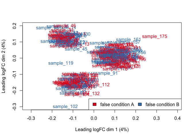
#Plot batch
plotMDS(y, col=cols[factor(groups$batch)])
legend(x = "bottomright", legend = paste("batch", 1:4), fill=cols, ncol=2)
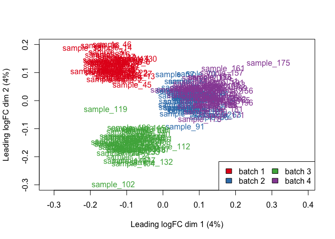
We can now apply the Supervised Normalisation of Microarrays method. A critical aspect of this approach is the incorporation of the variable of interest as an input, enhancing its capacity to preserve the associated signal. However, critically it assumes that there is not a correlation between the unwanted batch effects and the variable of interest. Thus, it is essential that the experimental design satisfies this condition. This is rarely the case in microbiome studies.
disease_matrix <- model.matrix(~disease_type, data=groups)
batch_matrix <- model.matrix(~batch, data=groups)

normalised <- snm(raw.dat = y,
                  bio.var = disease_matrix,
                  adj.var = batch_matrix,
                  rm.adj=TRUE,
                  verbose = TRUE,
                  diagnose = TRUE)
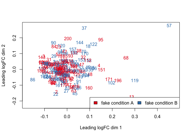
Let’s plot the results using Multidimensional Scaling (MDS).
plotMDS(normalised$norm.dat, col=cols[factor(groups$disease_type)],
        var.explained = FALSE)
legend(x = "bottomright", legend = c("fake condition A","fake condition B"), fill= cols, ncol=2)
plotMDS(normalised$norm.dat, col=cols[factor(groups$batch)],
        var.explained = FALSE)
legend(x = "bottomright", legend = paste("batch", 1:4), fill=cols, ncol=2)
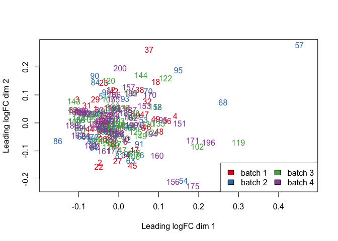
It’s handled the batch correction well and has not added any obvious artificial signal. However, things change when we add some correlation between the unwanted variation (batches) and the fake variable of interest.
To add some correlation between the groups and the ‘fake’ variable of interest, we can increase the probability a sample is of a particular cancer type if occurs within a subset of batches.
# a sample is 5 times more likely to be in condition 'b' if it belongs to an even batch number
fake_disease_type <- purrr::map_chr(as.numeric(factor(sim$Batch)),
                                    ~ sample(c('a','b'), size = 1, prob = c(1, 5*(.x %% 2))))

groups <- tibble(
  sample=paste('sample', 1:nsamples, sep="_"),
  batch = sim$Batch,
  disease_type=fake_disease_type
)

disease_matrix <- model.matrix(~disease_type, data=groups)
batch_matrix <- model.matrix(~batch, data=groups)

# account for read depth and transform to log space
y <- edgeR::cpm(count_matrix, normalized.lib.sizes = TRUE, log = TRUE, prior.count = 1)
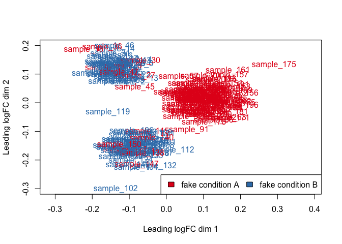
We can now check the un-normalised plots which look similar to before.
plotMDS(y, col=cols[factor(groups$disease_type)],
        var.explained = FALSE)
legend(x = "bottomright", legend = c("fake condition A","fake condition B"), fill= cols, ncol=2)
plotMDS(y, col=cols[factor(groups$batch)],
        var.explained = FALSE)
legend(x = "bottomright", legend = paste("batch", 1:4), fill=cols, ncol=2)

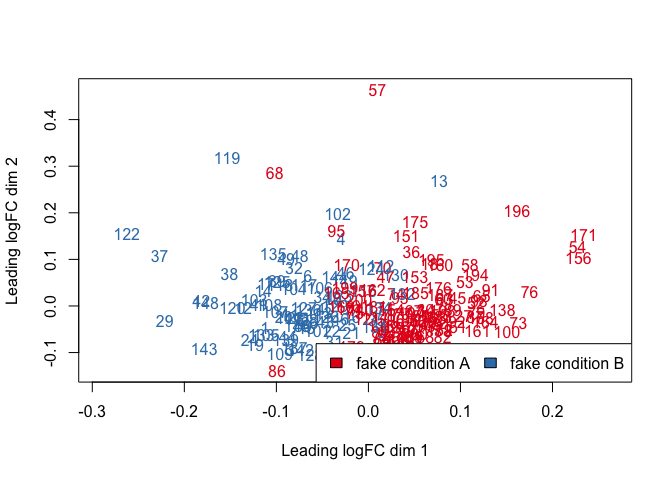
However, after normalisation, the data no longer clusters by batch. Instead, we see an unexpected clustering based on our simulated disease type!
normalised <- snm(raw.dat = y,
                  bio.var = disease_matrix,
                  adj.var = batch_matrix,
                  rm.adj=TRUE,
                  verbose = TRUE,
                  diagnose = TRUE)

plotMDS(normalised$norm.dat, col=cols[factor(groups$disease_type)],
        var.explained = FALSE)
legend(x = "bottomright", legend = c("fake condition A","fake condition B"), fill= cols, ncol=2)
plotMDS(normalised$norm.dat, col=cols[factor(groups$batch)],
        var.explained = FALSE)
legend(x = "bottomright", legend = paste("batch", 1:4), fill=cols, ncol=2)
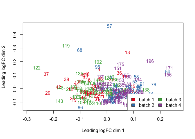
If we feed this imprinted data into a machine learning classifier, it will artificially increase its accuracy and incorrectly identify a signal associated with the fake variable of interest.
2: Accounting for unwanted variation in the TCGA data
Knowing that the supervised normalisation of microbiome data is problematic, I was interested in examining the signals present within the TCGA data and whether it was possible to account for the unwanted batch effects without imprinting the data with an artificial signal.
Although, the contamination with human reads has received a lot of attention, it seems unlikely that mutations in human genomes associated with cancer would result in sufficiently different contamination profiles to distinguish all cancer types. It should be possible to account for such contamination in the normalisation stage if suitable control samples are available.
To investigate this further, I was interested in whether the observed cancer correlations remained after we accounted for microbial variation observed in the corresponding tissue normal samples for each site.
These ‘normal’ samples are not an ideal control. If cancer associated bacteria are also present in the normal tissue this would remove such a signal. Ideally, we would have a corresponding set of body site specific normal tissue from patients without cancer. However, by using the normal tissue samples from the TCGA dataset we should be able to account for many batch effects including whether the observed correlations could simply be driven by site specific bacteria.
To start, lets load the original un-filtered count data from the original publication and the cleaned count data produced by Gihawi et al. in their recent preprint.
# Original counts with and without normalisation from Poore et al., 2020 https://www.nature.com/articles/s41586-020-2095-1
orignal_counts_raw <- read_csv("./data/Kraken-TCGA-Raw-Data-All-18116-Samples.csv")
colnames(orignal_counts_raw)[[1]] <- "Sample"
colnames(orignal_counts_raw) <- gsub(".*g__","",colnames(orignal_counts_raw))

meta_data <- read_csv("./data/tcga_metadata_poore_et_al_2020_1Aug23.csv")

meta_extra <- read_csv("./data/Metadata-TCGA-All-18116-Samples.csv")
colnames(meta_extra)[[1]] <- "Sample"

meta_data$gender <- meta_extra$gender[match(meta_data$sampleid, meta_extra$Sample)]
meta_data$platform <- meta_extra$platform[match(meta_data$sampleid, meta_extra$Sample)]
meta_data$portion_ffpe <- meta_extra$portion_is_ffpe[match(meta_data$sampleid, meta_extra$Sample)]
meta_data$experimental_strategy <- meta_extra$experimental_strategy[match(meta_data$sampleid, meta_extra$Sample)]
meta_data$tissue_source_site_label <- meta_extra$tissue_source_site_label[match(meta_data$sampleid, meta_extra$Sample)]


#Load the updated counts from Gihawi et al., bioRxiv 2023.  https://github.com/yge15/Cancer_Microbiome_Reanalyzed
gihawi_counts <- map(c("./data/TableS8_BLCA.all.csv", "./data/TableS9_HNSC_all.csv", "./data/TableS10_BRCA_WGS.csv"), ~ {
                       df <- read_csv(.x)
                      colnames(df)[[1]] <- "Sample"
                      colnames(df) <- gsub("^g_","",colnames(df))
                      return(df)
                     })
common_species <- Reduce(intersect, map(gihawi_counts, colnames))
common_species <- common_species[common_species!="Homo"] # remove human reads

gihawi_counts <- map_dfr(gihawi_counts, ~ .x[,common_species])

#subset metadata and samples
meta_data <- meta_data[meta_data$sampleid %in% gihawi_counts$Sample,]
orignal_counts_raw <- orignal_counts_raw[orignal_counts_raw$Sample %in% gihawi_counts$Sample, ]
orignal_counts_raw <- orignal_counts_raw[, c(TRUE, colSums(orignal_counts_raw[,2:ncol(orignal_counts_raw)]))>0]

# Order all matrices to match the meta table
gihawi_counts <- gihawi_counts[match(meta_data$sampleid, gihawi_counts$Sample),]
orignal_counts_raw <- orignal_counts_raw[match(meta_data$sampleid, orignal_counts_raw$Sample),]
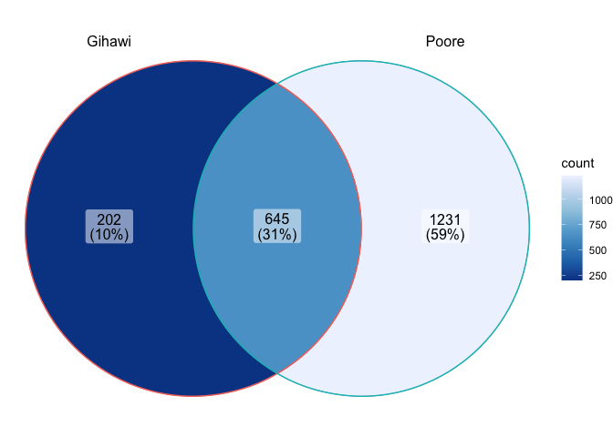
We can consider the intersection between the species observed in the original un-filtered data and the cleaned set from the preprint.
ggVennDiagram::ggVennDiagram(list(Gihawi=colnames(gihawi_counts)[-1],
                                  Poore=colnames(orignal_counts_raw)[-1])) +
  scale_fill_distiller(palette = 1)
2.1 Analysis of Gihawi et al. filtered counts
In a response to the Gihawi et al. pre-print, Poore et al. identified a cancer-specific microbial signature in a subset of the TCGA data, which included three cancer types sequenced at Harvard Medical School. To tackle the issue of normalisation, they utilised the cleaned counts from Gihawi et al., without implementing any normalisation procedures.
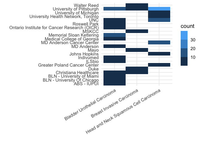
While all samples were processed at HMS, they originated from different hospitals and included cancers from different body sites. Thus, it is not clear if the identified signal was due to the cancer type or remaining batch effects.
Indeed, if we create an MDS plot of this data we observe quite clear clusters.
filt_meta <- meta_data %>%
  filter(!grepl(".*Normal", sample_type)) %>%
  filter(data_submitting_center_label=="Harvard Medical School")

filt_counts <- gihawi_counts[gihawi_counts$Sample %in% filt_meta$sampleid, ]

stopifnot(all(filt_counts$Sample==filt_meta$sampleid))

filt_counts <- t(filt_counts[,-1])
colnames(filt_counts) <- filt_meta$sampleid

filt_counts <- filt_counts[, colSums(filt_counts)>100]
filt_meta <- meta_data[meta_data$sampleid %in% colnames(filt_counts), ]

y <- edgeR::cpm(filt_counts, normalized.lib.sizes = TRUE, log = TRUE, prior.count = 1)

plotMDS(y, col=cols[factor(filt_meta$disease_type)],
        var.explained = FALSE)
legend(x = "bottomright", legend = unique(filt_meta$disease_type), fill=rev(cols[1:3]), ncol=1)
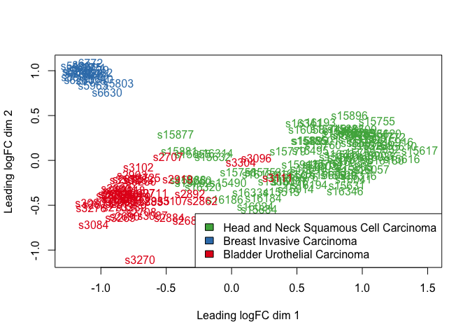
However, while the sequencing center is the same, other potential batch effects could be driving the signal including the hospital the samples originated from and the body site the cancer was located in. We can plot the distribution of cancer types by hospital.
ggplot(filt_meta, aes(x=disease_type, y=tissue_source_site_label)) +
  geom_bin2d() +
  theme_minimal(base_size = 14) +
  theme(axis.text.x = element_text(angle = 30, hjust = 1)) +
  scale_fill_binned() +
  xlab("") + ylab("")
One option to account for these sources of unwanted variation is to use the associated non-cancer normal tissue samples as controls. We can use the excellent SCRuB decontamination method to do this.
As there are no normal tissue samples for the breast cancer samples at Harvard Medical School we restrict this analysis to the remaining two cancer types.
First, let’s check the number of remaining reads in each sample
filt_meta <- meta_data %>%
  filter(data_submitting_center_label=="Harvard Medical School") %>%
  filter(sample_type!="Blood Derived Normal")

# split into normal and cancerous tissue samples
filt_meta$normal <- grepl(".*Normal", filt_meta$sample_type)

# Keep those where we have both tumor and normal tissue samples.
keep <- filt_meta %>%
  group_by(investigation, data_submitting_center_label) %>%
  dplyr::summarise(
    normal_and_cancer = length(unique(normal))>1,
    n_normal = sum(normal),
    n_cancer = sum(!normal)
  ) %>% filter(normal_and_cancer)

filt_meta <- filt_meta %>%
  filter(paste(investigation, data_submitting_center_label) %in% paste(keep$investigation, keep$data_submitting_center_label))

filt_counts <- gihawi_counts[gihawi_counts$Sample %in% filt_meta$sampleid, ]
stopifnot(all(filt_counts$Sample==filt_meta$sampleid))

filt_counts <- t(filt_counts[,-1])
colnames(filt_counts) <- filt_meta$sampleid

pdf <- tibble(
  `cancer type`=filt_meta$disease_type,
  `number of reads` = colSums(filt_counts)
)

ggplot(pdf, aes(x=`cancer type`, y=`number of reads`, colour=`cancer type`)) +
  geom_boxplot(outlier.colour = NA) +
  ggbeeswarm::geom_quasirandom() +
  scale_y_log10() +
  scale_color_manual(values = cols[-2]) +
  theme_minimal(base_size = 14) +
  theme(legend.position = 'none') +
  xlab("")
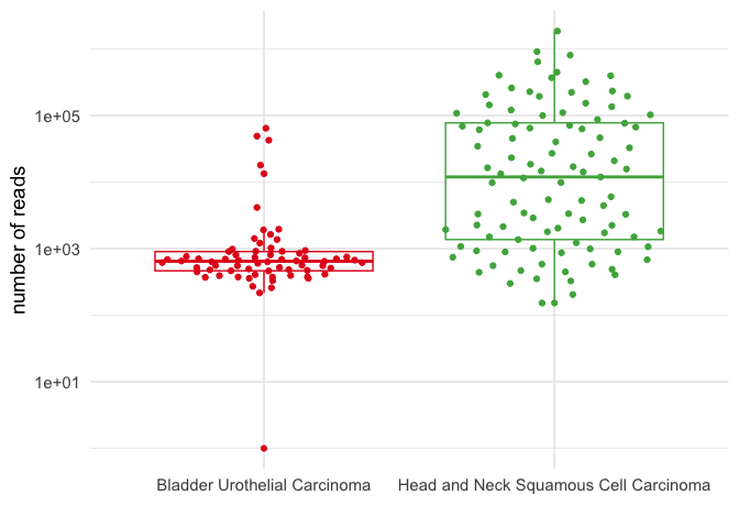
The number of microbial reads vary substantially by cancer type. While it might be possible to account for some of this by normalising for total read counts, it is unlikely to account for the increased number of potential species that could be observed at much higher read depths.
Instead, we restrict out analysis to samples with similar read counts of between 500 and 50,000 reads.
# Throw out samples with < 100 reads
filt_counts <- filt_counts[, (colSums(filt_counts)>500) & (colSums(filt_counts)<50000)]
filt_meta <- filt_meta[filt_meta$sampleid %in% colnames(filt_counts), ]

# Run the SCRuB algorithm on each cancer type
scrub_counts <- purrr::map2(keep$data_submitting_center_label, keep$investigation, ~{
  # print(paste(.x, .y, sep = " : "))

  k <- (filt_meta$investigation==.y) & (filt_meta$data_submitting_center_label==.x)

  case_counts <- t(filt_counts[, k & !filt_meta$normal])
  control_counts <- t(filt_counts[, k & filt_meta$normal])

  new_meta <- filt_meta[k,] %>%
    filter(!normal)

  # Account for site specific signatures using SCruB
  norm_counts <- t(SCRUB_no_spatial(case_counts, control_counts)$decontaminated_samples)

  stopifnot(all(colnames(norm_counts)==new_meta$sampleid))

  return(list(norm_counts=norm_counts, meta=new_meta))
})

scrub_meta <- map_dfr(scrub_counts, ~ .x$meta)
scrub_counts <- do.call(cbind, purrr::map(scrub_counts, ~ .x$norm_counts))

# Account for remaining unwanted variables including gender and the hospital where the sample was taken
y <- edgeR::cpm(scrub_counts, normalized.lib.sizes = TRUE, log = TRUE, prior.count = 1)

plotMDS(y, col=cols[-2][factor(scrub_meta$disease_type)],
        var.explained = FALSE)
legend(x = "bottomright", legend = unique(scrub_meta$disease_type), fill=cols[-2], ncol=1)
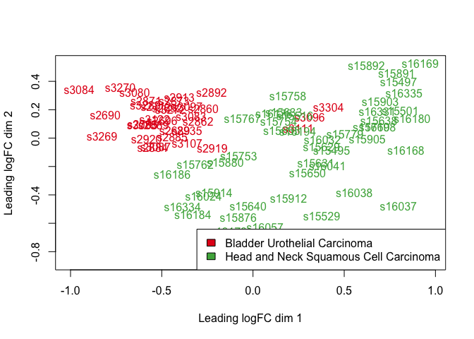
Once body site-specific microbial signatures are accounted for, the distinction between cancer types diminishes slightly. However, if we factor in the hospital from which samples were collected—a potential source of contamination—no obvious signal remains.
y <- removeBatchEffect(y, batch = scrub_meta$tissue_source_site_label)

plotMDS(y, col=cols[-2][factor(scrub_meta$disease_type)],
        var.explained = FALSE)
legend(x = "bottomright", legend = unique(scrub_meta$disease_type), fill=cols[-2], ncol=1)
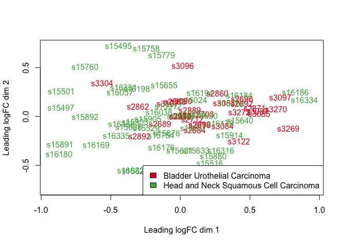
So far, we have shown that Supervised Normalisation can artificially imprint a data set with a signal if there is a correlation between the variable of interest and unwanted batch effects.
After employing rigorous normalisation methods to mitigate potential influences from body site and hospital batch effects, the distinction between Bladder Urothelial Carcinoma and Head and Neck Squamous Cell Carcinoma isn’t evident. While this doesn’t rule out unique microbial signatures in these samples, the TCGA study design complicates the task of detecting a robust signal.
2.2 Analysis of the original Poore et al. read counts
As we can use alternative normalisation strategies to account for batch effects within the TCGA data, I was interested in whether these would work on the original count data from the Poore et al., paper.
This presupposes that any cancer-associated human contaminant reads, as identified in the Gihawi et al. preprint, are unlikely to align with different bacterial species compared to non-cancerous human reads.
To investigate this, I started by considering the same samples sequenced at Harvard Medical School.
filt_meta <- meta_data %>%
  filter(data_submitting_center_label=="Harvard Medical School") %>%
  filter(sample_type!="Blood Derived Normal")

# split into normal and cancerous tissue samples
filt_meta$normal <- grepl(".*Normal", filt_meta$sample_type)

# Keep those where we have both tumor and normal tissue samples.
keep <- filt_meta %>%
  group_by(investigation, data_submitting_center_label) %>%
  dplyr::summarise(
    normal_and_cancer = length(unique(normal))>1,
    n_normal = sum(normal),
    n_cancer = sum(!normal)
  ) %>% filter(normal_and_cancer)

filt_meta <- filt_meta %>%
  filter(paste(investigation, data_submitting_center_label) %in% paste(keep$investigation, keep$data_submitting_center_label))

filt_counts <- orignal_counts_raw[orignal_counts_raw$Sample %in% filt_meta$sampleid, ]
stopifnot(all(filt_counts$Sample==filt_meta$sampleid))

filt_counts <- t(filt_counts[,-1])
colnames(filt_counts) <- filt_meta$sampleid

filt_meta <- filt_meta[filt_meta$sampleid %in% colnames(filt_counts), ]

# Run the SCRuB algorithm on each cancer type
scrub_counts <- purrr::map2(keep$data_submitting_center_label, keep$investigation, ~{
  # print(paste(.x, .y, sep = " : "))

  k <- (filt_meta$investigation==.y) & (filt_meta$data_submitting_center_label==.x)

  case_counts <- t(filt_counts[, k & !filt_meta$normal])
  control_counts <- t(filt_counts[, k & filt_meta$normal])

  new_meta <- filt_meta[k,] %>%
    filter(!normal)

  # Account for site specific signatures using SCruB
  norm_counts <- t(SCRUB_no_spatial(case_counts, control_counts)$decontaminated_samples)

  stopifnot(all(colnames(norm_counts)==new_meta$sampleid))

  return(list(norm_counts=norm_counts, meta=new_meta))
})

scrub_meta <- map_dfr(scrub_counts, ~ .x$meta)
scrub_counts <- do.call(cbind, purrr::map(scrub_counts, ~ .x$norm_counts))
As the read counts are now much higher and similar between cancer types we do not need to filter out samples by read depth prior to running SCRuB.
However, the SCRuB algorithm now assigns the vast majority of read counts to potential contamination. This demonstrates that using good control samples when performing normalisation and batch correction can account for even large issues with contamination, as long as that contamination is not correlated with the variable of interest.
We can look at the difference in read counts before and after using a log-scaled plot.
pdf <- tibble(
       sample=colnames(scrub_counts),
       center=scrub_meta$data_submitting_center_label,
       cancer_type=scrub_meta$disease_type,
       `Original un-filtered counts`=colSums(filt_counts)[match(colnames(scrub_counts), colnames(filt_counts))],
       `Counts after SCRuB normalisation`=colSums(scrub_counts)) %>%
  pivot_longer(cols=c("Original un-filtered counts","Counts after SCRuB normalisation"))

ggplot(pdf, aes(x=sample, y=value, colour=name)) +
  geom_point() +
  # scale_y_log10() +
  scale_y_continuous(trans=scales::pseudo_log_trans(base = 10),
                     breaks=c(0, 10, 100,1000,1e4,1e5,1e6,1e7)) +
  facet_wrap(~cancer_type, scales = "free_x") +
  scale_color_brewer(type = 'q', palette = 2) +
  theme_minimal(base_size = 14) +
  theme(axis.text.x=element_blank(),
        axis.ticks.x=element_blank(),
        legend.position="bottom",
        legend.title=element_blank()) +
  ylab("Total read count (log scale)")
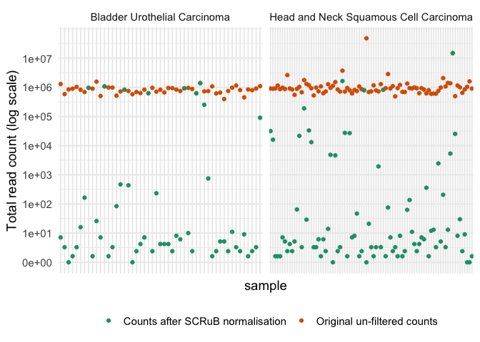
After filtering out signals present in the tissue normal samples, some samples have very low read depths making them unsuitable for further analysis. After filtering these out, we can look at how the remaining samples cluster together.
# Throw out samples with < 100 reads
scrub_counts <- scrub_counts[, colSums(scrub_counts)>100]
scrub_meta <- scrub_meta[scrub_meta$sampleid %in% colnames(scrub_counts), ]

# Account for remaining unwanted variables including gender and the hospital where the sample was taken
y <- edgeR::cpm(scrub_counts, normalized.lib.sizes = TRUE, log = TRUE, prior.count = 1)

plotMDS(y, col=cols[-2][factor(scrub_meta$disease_type)],
        var.explained = FALSE)
legend(x = "bottomright", legend = unique(scrub_meta$disease_type), fill=cols[-2], ncol=1)
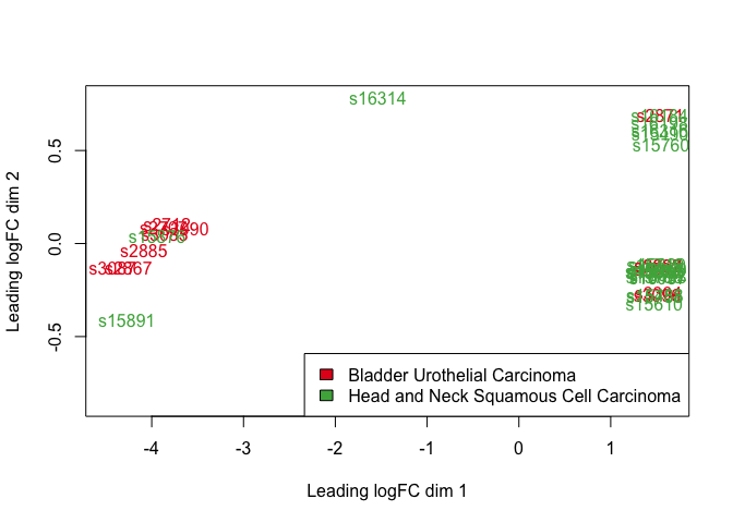
There is no longer any clustering by cancer type, but there does appear to be some clustering driven by a remaining batch effect. Accounting for the hospital removes this effect.
y <- removeBatchEffect(y, batch = scrub_meta$tissue_source_site_label)

plotMDS(y, col=cols[-2][factor(scrub_meta$disease_type)],
        var.explained = FALSE)
legend(x = "bottomright", legend = unique(scrub_meta$disease_type), fill=cols[-2], ncol=1)
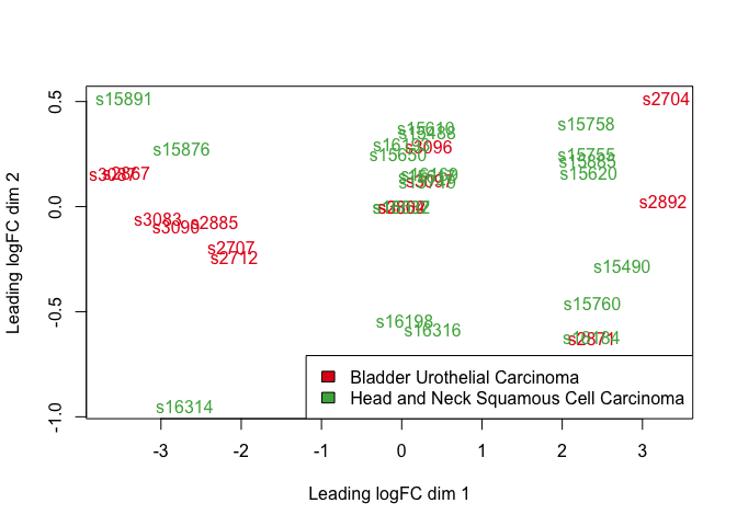
While it is always better to start with cleaner data, this analysis demonstrates that a careful use of normalisation and batch correction techniques can help to correct for even large amounts of contamination.
As we have shown that we can account for most unwanted variation in the subset of samples from Harvard, even when using the original un-filtered count data, we can now investigate the signals present in the larger dataset originally published by Poore et al.
3. Re-analysis of Poore et al. data across hospital sites and cancer types
To start, I load the full unfiltered TCGA data from the Poore et al., manuscript.
To streamline the analysis and avoid some undesired variables, I’ve limited the re-analysis to WGS samples sequenced using the Illumina HiSeq.
In order to implementation of the SCRuB algorithm, I further restrict the analysis to consider only those cancer type and sequencing institute pairings that have a minimum of three cancer tissue samples and three normal tissue control samples.
This results in a data set of 1,809 cancer samples across 16 cancer types.
meta_data <- read_csv("./data/tcga_metadata_poore_et_al_2020_1Aug23.csv")
meta_extra <- read_csv("./data/Metadata-TCGA-All-18116-Samples.csv")
colnames(meta_extra)[[1]] <- "Sample"

meta_data$gender <- meta_extra$gender[match(meta_data$sampleid, meta_extra$Sample)]
meta_data$platform <- meta_extra$platform[match(meta_data$sampleid, meta_extra$Sample)]
meta_data$portion_ffpe <- meta_extra$portion_is_ffpe[match(meta_data$sampleid, meta_extra$Sample)]
meta_data$experimental_strategy <- meta_extra$experimental_strategy[match(meta_data$sampleid, meta_extra$Sample)]
meta_data$tissue_source_site_label <- meta_extra$tissue_source_site_label[match(meta_data$sampleid, meta_extra$Sample)]

orignal_counts_raw <- read_csv("./data/Kraken-TCGA-Raw-Data-All-18116-Samples.csv")
colnames(orignal_counts_raw)[[1]] <- "Sample"
colnames(orignal_counts_raw) <- gsub(".*g__","",colnames(orignal_counts_raw))

meta_data <- meta_data[match(orignal_counts_raw$Sample, meta_data$sampleid), ]

filt_meta <- meta_data %>%
  filter(sample_type!="Blood Derived Normal") %>%
  filter(platform=='Illumina HiSeq') %>%
  filter(portion_ffpe=='NO') %>%
  filter(experimental_strategy=='WGS')

# split into normal and cancerous tissue samples
filt_meta$normal <- grepl(".*Normal", filt_meta$sample_type)

# Keep those where we have both tumor and at least 3 normal tissue samples.
keep <- filt_meta %>%
  group_by(investigation, data_submitting_center_label) %>%
  dplyr::summarise(
    normal_and_cancer = length(unique(normal))>1,
    n_normal = sum(normal),
    n_cancer = sum(!normal)
  ) %>%
  filter(n_normal>3) %>%
  filter(n_cancer>3)

filt_meta <- filt_meta %>%
  filter(paste(investigation, data_submitting_center_label) %in% paste(keep$investigation, keep$data_submitting_center_label))

filt_counts <- orignal_counts_raw[orignal_counts_raw$Sample %in% filt_meta$sampleid, ]
stopifnot(all(filt_counts$Sample==filt_meta$sampleid))

filt_counts <- t(filt_counts[,-1])
colnames(filt_counts) <- filt_meta$sampleid

filt_meta <- filt_meta[filt_meta$sampleid %in% colnames(filt_counts), ]

# Run the SCRuB algorithm on each cancer type
scrub_counts <- purrr::map2(keep$data_submitting_center_label, keep$investigation, ~{
  # print(paste(.x, .y, sep = " : "))

  k <- (filt_meta$investigation==.y) & (filt_meta$data_submitting_center_label==.x)

  case_counts <- t(filt_counts[, k & !filt_meta$normal])
  control_counts <- t(filt_counts[, k & filt_meta$normal])

  new_meta <- filt_meta[k,] %>%
    filter(!normal)

  # Account for site specific signatures using SCruB
  norm_counts <- t(SCRUB_no_spatial(case_counts, control_counts)$decontaminated_samples)

  stopifnot(all(colnames(norm_counts)==new_meta$sampleid))

  return(list(norm_counts=norm_counts, meta=new_meta))
})

scrub_meta <- map_dfr(scrub_counts, ~ .x$meta)
scrub_counts <- do.call(cbind, purrr::map(scrub_counts, ~ .x$norm_counts))

# Throw out samples with < 100 reads and species with < 10
scrub_counts <- scrub_counts[, colSums(scrub_counts)>100]
scrub_counts <- scrub_counts[rowSums(scrub_counts)>10, ]
scrub_meta <- scrub_meta[scrub_meta$sampleid %in% colnames(scrub_counts), ]
We can now generate some plots to look for evidence of clustering by type across a much larger subset of 1,809 samples from the TCGA data set
y <- edgeR::cpm(scrub_counts, normalized.lib.sizes = TRUE, log = TRUE, prior.count = 1)

# Account for remaining unwanted variables including gender and the hospital where the sample was taken
y <- removeBatchEffect(y, batch = scrub_meta$tissue_source_site_label)

pca_res <- prcomp(y)

pdf <- cbind(scrub_meta, pca_res$rotation[,1:10])

ggplot(pdf, aes(x=PC1, y=PC2, col=disease_type, shape=disease_type)) +
  geom_point() +
  scale_shape_manual(values =1:17) +
  theme_minimal(base_size = 14) +
  labs(colour="Cancer type") +
  labs(shape="Cancer type")
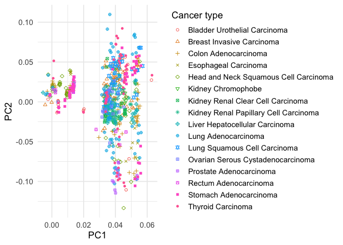
There appears to be a clustering along the first principal component. However, this was not correlated with cancer type or any of the other unwanted variables available in the metadata.
We can also consider a t-SNE plot which can sometimes reveal fine scale structure in high dimensional data sets.
tsne <- Rtsne::Rtsne(pca_res$rotation[,1:50], pca=FALSE, perplexity=50, check_duplicates=FALSE)
colnames(tsne$Y) <- paste('TSNE dim', 1:ncol(tsne$Y))

pdf <- cbind(scrub_meta, tsne$Y)

ggplot(pdf, aes(x=`TSNE dim 1`, y=`TSNE dim 2`, col=disease_type, shape=disease_type)) +
  geom_point() +
  scale_shape_manual(values =1:17) +
  theme_minimal(base_size = 14) +
  labs(colour="Cancer type") +
  labs(shape="Cancer type")
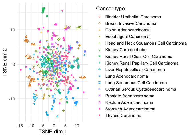
Again, although there appears to be some clustering it does not correlate strongly with cancer type.
Finally, an alternative method for determining if there is cancer associated clusters within this data is to build a machine learning model and estimate how accurately it can identify cancer types.
Here, I used the same Gradient Boosted Trees method as was used in the rebuttal to the preprint by Gihawi et al.
# Set up data sets and set seed
set.seed(1234)
trainX <- t(scrub_counts)
trainY <-  factor(gsub("^TCGA-","", scrub_meta$investigation))

# Set up model
xgbGrid <- data.frame(nrounds = 10,
                      max_depth = 4,
                      eta = .1,
                      gamma = 0,
                      colsample_bytree = .7,
                      min_child_weight = 1,
                      subsample = .8)


# as ctrl defines the cross validation sampling during training
ctrl <- trainControl(method = "repeatedcv",
                     number = 10,
                     repeats = 1,
                     sampling = "up",
                     summaryFunction = multiClassSummary,
                     classProbs = TRUE,
                     verboseIter = FALSE,
                     savePredictions = TRUE,
                     allowParallel=TRUE)

set.seed(1234)
mlModel <- train(x = trainX,
                 y = trainY,
                 method = "xgbTree",
                 nthread = 1,
                 trControl = trainControl(method = "repeatedcv",
                                          number = 10,
                                          repeats = 1,
                                          sampling = "up",
                                          summaryFunction = multiClassSummary,
                                          classProbs = TRUE,
                                          verboseIter = FALSE,
                                          savePredictions = TRUE,
                                          allowParallel=TRUE),
                 tuneGrid = xgbGrid,
                 verbose = FALSE)


conf <- confusionMatrix(data = mlModel$pred$pred, reference = trainY, mode = "prec_recall")

conf$overall
##       Accuracy          Kappa  AccuracyLower  AccuracyUpper   AccuracyNull
##     0.06090652    -0.01140231     0.04442535     0.08116699     0.11331445
## AccuracyPValue  McnemarPValue
##     0.99999930            NaN
After controlling for sampling site and other unwanted batch effects, the machine learning model achieved an accuracy of 0.0609065 which is not significantly more than a null model.
Our approach to normalisation has been quite strict, so this analysis does not rule out an association between microbial reads and cancer types in this data set. In fact, due to the correlation between unwanted batch effects and cancer type it is challenging to identify robust microbial signatures associated with cancer in the TCGA data set.
However, it does indicate that by using appropriate normalisation techniques we are able to account for problems with contamination and database errors.
In the future, careful study designs that include body site specific but non-cancerous controls are necessary to accurately identify association between microbial DNA and cancer types.
Ultimately, to ascertain whether microbial DNA signatures can be utilised in cancer diagnostics, large comprehensive trials encompassing both cancer-afflicted and healthy patients will be required.
Acknowledgements
Thanks to Prof. Lachlan Coin for helpful advice and comments.
References
Sepich-Poore G. tcga_rebuttal: Re-analysis of data provided by Gihawi et al. 2023 bioRxiv. Github; Available: https://github.com/gregpoore/tcga_rebuttal
Gihawi A, Ge Y, Lu J, Puiu D, Xu A, Cooper CS, et al. Major data analysis errors invalidate cancer microbiome findings. bioRxiv. 2023. p. 2023.07.28.550993. doi:10.1101/2023.07.28.550993
Sepich-Poore GD, Kopylova E, Zhu Q, Carpenter C, Fraraccio S, Wandro S, et al. Reply to: Caution Regarding the Specificities of Pan-Cancer Microbial Structure. bioRxiv. 2023. p. 2023.02.10.528049. doi:10.1101/2023.02.10.528049
Gihawi A, Cooper CS, Brewer DS. Caution Regarding the Specificities of Pan-Cancer Microbial Structure. bioRxiv. 2023. p. 2023.01.16.523562. doi:10.1101/2023.01.16.523562
Austin GI, Park H, Meydan Y, Seeram D, Sezin T, Lou YC, et al. Contamination source modeling with SCRuB improves cancer phenotype prediction from microbiome data. Nat Biotechnol. 2023. doi:10.1038/s41587-023-01696-w
Poore GD, Kopylova E, Zhu Q, Carpenter C, Fraraccio S, Wandro S, et al. Microbiome analyses of blood and tissues suggest cancer diagnostic approach. Nature. 2020;579: 567–574. doi:10.1038/s41586-020-2095-1
Wang Y, LêCao K-A. Managing batch effects in microbiome data. Brief Bioinform. 2020;21: 1954–1970. doi:10.1093/bib/bbz105
Zappia L, Phipson B, Oshlack A. Splatter: simulation of single-cell RNA sequencing data. Genome Biol. 2017;18: 174. doi:10.1186/s13059-017-1305-0
Mecham BH, Nelson PS, Storey JD. Supervised normalization of microarrays. Bioinformatics. 2010;26: 1308–1315. doi:10.1093/bioinformatics/btq118
